Today, let’s dive into an interesting approach to trading using the k-nearest neighbors (KNN) algorithm. This method acts like a memory-based machine learning technique, though I must admit, my initial attempts didn’t quite hit the mark. Whether it was due to insufficient tinkering or a lack of deeper understanding, I figured it was worth sharing for discussion and improvement.
The heart of this method lies in the Euclidean_Metric function, which serves as a classifier. Essentially, it uses a vector base that describes trades or market conditions to determine if an input vector fits into any predefined groups. In simple terms, if a trade wraps up with a profit, it gets classified as class 1; if it’s a loss, that’s class 0. The classifier then looks for the nearest neighbors of a multi-dimensional vector using Euclidean distance. It counts how many of these k vectors belong to class 1, divides that by k, and voilà—there’s your probability of that vector being a winning trade. However, because we might not always pick the best vector coordinates, we can’t fully rely on this classification alone. To add a safety net, I introduced an additional threshold: if the probability of a profitable trade is over 0.7, then it’s time to jump in!
We use the ratios of moving averages as the measures (or coordinates) in this setup. The idea is that once we classify the trades, we can leverage that classification in future tests. But, as with many things in trading, it’s not as straightforward as it sounds! Why choose k-nearest neighbors? It’s primarily because the first nearest neighbor can sometimes be an outlier, leading us astray without considering that there may be a cluster of contrary vectors nearby. For a more detailed look into this, check out S. Haykin’s book, Neural Networks: A Comprehensive Foundation.
Challenges Faced
This classifier comes with a couple of hurdles:
- 1) Finding a reliable static dataset that accurately describes market situations or potential trades.
- 2) The hefty volume of mathematical operations required, which can slow down computations (though it’s marginally faster than PNN).
To put it simply, these issues mirror those found in traditional trading systems. The upside is that this classifier can formalize conditions that traders might not consciously notice but can feel intuitively affect their trading decisions.
Implementation Insights
Let’s get into the nitty-gritty of how to implement this:
- Base - Set to true to write a vector file, or false to engage in trade classification.
- buy_threshold = 0.6: This is the threshold for all buy positions.
- sell_threshold = 0.6: The same applies for sell trades.
- inverse_position_open = true: If the probability of a profitable trade is low, why not consider entering the market with an inverted position? This flag allows that.
- inverse_buy_threshold = 0.3: If the probability of a profitable buy is lower than this threshold, open a sell trade.
- inverse_sell_threshold = 0.3: Likewise for sell trades.
- fast = 12: These are the MACD parameters.
- slow = 34;
- tp = 40: Your take profit parameter.
- sl = 30: Your stop loss parameter.
- close_orders = false: This flag allows for closing positions only when there’s an opposite signal and the order is in profit.
Here’s how to use it: First, set Base to true, adjust sl to equal tp, and run it on historical data just once to generate your vector file. Next, switch Base to false and optimize your thresholds based on your first report (without classification). If you see a success probability of 0.5, set your thresholds to 0.6 for entry and 0.4 for an inverted position.
This is just an example; you can adapt the classifier for other trading systems using different input data.
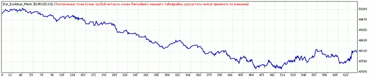
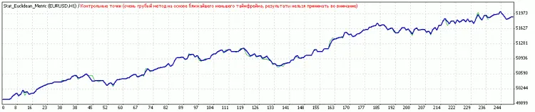
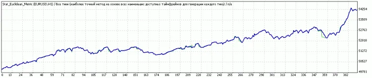
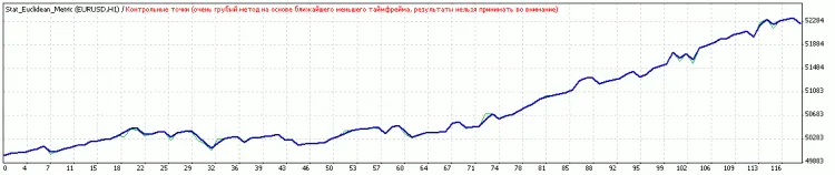
Visuals and Results
Let’s take a look at the performance before and after optimization:
After optimization of thresholds:


Comments 0